This is part four of a series on statistical methods for analysing time-to-event, or "survival" data.
Key takeaways
- Competing risks occur when individuals can experience multiple possible events that prevent the observation of other events
- Standard survival methods (Kaplan-Meier, Cox) can produce biased estimates when competing risks are present
- The cause-specific hazard function measures the instantaneous risk of a specific event type
- The cause-specific cumulative incidence function gives the probability of experiencing a specific event type over time
- The Aalen-Johansen estimator is the non-parametric method for estimating cumulative incidence in competing risks scenarios
- The Fine-Gray model allows regression analysis for competing risks data by modeling the sub-distribution hazard
- Stratification can accommodate non-proportional hazards in both Cox and Fine-Gray models
Competing risks
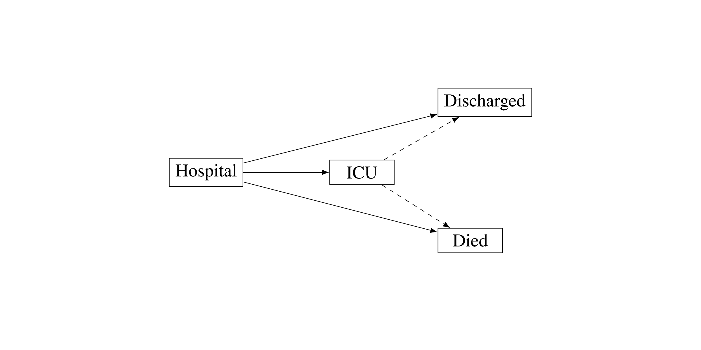
In medical cohort studies, multiple study end-points are common (e.g. death, intensive care admission, and discharge). These multiple end-points are known as competing risks and may hinder the event of interest, or modify the chance that this event occurs. Kaplan-Meier and Cox proportional hazards models treat competing risks as censored observations, and do not account for dependencies between events. Hence the assumption of independent times-to-events in these conventional survival analyses is violated in the presence of competing risks.
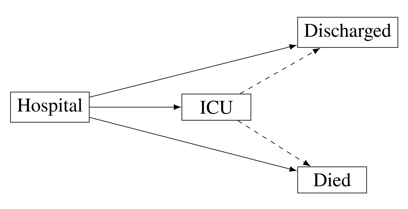
Figure 1: Example of competing risks (death, discharge, and intensive care (ICU) admission) in hospital survival data.
To correctly address competing risks, "competing risks survival models" are available. In these models an individual is observed over time, with several possible events 'competing' until one takes place and the individual transitions to the corresponding state. Importantly there is no assumption of independence for the distribution of the time to competing events and censoring can still be appropriately accounted for.
Cause-specific survival functions
We'll start by defining the cause-specific hazard and cause-specific cumulative incidence functions, which are the key components of competing risks survival analysis.
Cause-specific hazard function
Let $T$ be a random variable for the survival time and $C$ be a random variable for the cause of failure. The cause-specific hazard function for the $j$th cause, $j = \{1, 2, \ldots, m\}$ is defined by:
$$h_j(t) = \lim_{\delta t \downarrow 0} \frac{\Pr(t \leq T < t + \delta t, C=j \mid T \geq t)}{\delta t} $$
Defining $f_j(t)$ as the cause-specific density function, and $S(t)=\Pr(T \geq t)$ as the overall survivor function, the relationship shown in part II of this series still holds in the presence of competing risks:
$$h_j(t)=\frac{f_j(t)}{S(t)}$$
Cause-specific cumulative incidence
The cause-specific cumulative incidence function, i.e. the probability of surviving until time $t$ and failure from cause $j$, in the presence of all other risks, is given by:
$$F_j(t) = \Pr(T < t, C=j)$$
for $j=\{1, 2, \dots, m\}$, with $\Pr(C=j)$ often written as $\pi_j$. An expression for $F_j(t)$ in terms of the cause-specific hazard function may be derived using the equation above:
$$\begin{aligned} h_j(t) &=\frac{f_j(t)}{S(t)} \\ f_j(t) &=S(t)h_j(t) \\ F_j(t) &=\int_0^t S(u)h_j(u) du \end{aligned}$$
Aalen-Johansen estimator
The standard non-parametric estimator of the cause-specific incidence function is the Aalen-Johansen estimator, also described as the 'multi-state version' of the Kaplan-Meier estimator.
Firstly, by the non-parametric Nelson-Aalen estimator of the cause-specific hazard function for cause $j$:
$$\hat{h}_j(t) = \frac{d_{j}(t)}{n(t\mbox{-})}$$
where $d_{j}(t)$ is the number of deaths due to cause $j$ at time $t$, and $n(t\mbox{-})$ is the number of individuals at risk just prior to $t$.
With the Kaplan-Meier estimate of the survivor function defined in part III of this series, $\hat{S}(t)$, the Aalen-Johansen estimator for the cause-specific cumulative incidence function then follows from the equation above:
$$\hat{F}_j(t) = \sum_{t_k < t} \hat{S}(t_{k-1})\frac{d_{j}(t_k)}{n(t_k\mbox{-})} $$
for all times $t_k < t$ where transition events are observed to occur.
Fine-Gray proportional hazards model
Analogous to the Cox proportional hazards model described in the last post, the Fine-Gray proportional hazards model may be used estimate the hazard of a competing event (termed the sub-distribution hazard) among those yet to experience an event by time $t$. The risk set for the sub-distribution hazard consists of both those who have yet to experience any event, and those who have yet to experience the event of interest, but who have experienced a competing event.
Sub-distribution hazard
The sub-distribution hazard is therefore defined as the instantaneous risk of experiencing a competing event $j$ given that the individual has not already experienced this event:
$$ \lambda_j(t)=\lim_{\delta t \downarrow 0}{\left\{\frac{\Pr\left(\left[t \leq T < t + \delta t, C=j \mid (T>t)\right] \cup \left[(T \le t \cap C \neq j)\right]\right)}{\delta t}\right\}} $$
where, as before, $C$ is the random variable for the event that occurs.
Fine-Gray regression
Fine-Gray regression links the sub-distribution hazard, $\lambda_{j}$, to the cause-specific cumulative incidence function, $F_{j}$, through the relationship:
$$ \lambda_{j}(t) = - \frac{d}{dt} \log{(1-F_{j}(t))} $$
As with the Cox proportional hazards model, a proportional hazards regression model is assumed, where the hazard of cause $j$ at time $t$ for individual $i$ is:
$$ \lambda_{i,j}(t) = \exp(\boldsymbol{\beta}^\mathsf{T}\boldsymbol{z}_i)\lambda^{(0)}_{j}(t) $$
with $\lambda^{(0)}_{j}(t)$ being the baseline sub-distribution hazard for cause $j$. Covariate coefficients are estimated by maximising the weighted partial likelihood $L(\boldsymbol{\beta})$:
$$ L(\boldsymbol{\beta}) = \prod_{i \in D}\frac{\exp(\boldsymbol{\beta}^\mathsf{T}\boldsymbol{z}_{d_i})}{\sum_{j \in R_i}w_{i,j}\exp(\boldsymbol{\beta}^\mathsf{T}\boldsymbol{z}_j)} $$
where $w_{i,j}$ are weights which account for the increasing probability of censoring with increasing follow-up time, $D = \{T_1, T_2, \ldots, T_n\}$ are the set of distinct failure times, $R_i$ is the set of all individuals who are at risk of failure immediately before time $T_i$, $\boldsymbol{z}_{d_i}$ is the covariate vector for an individual who failed at time $T_i$, and $\boldsymbol{z}_j$ is the covariate vector for the $j$th individual at risk at time $T_i$. Covariate effects on the sub-distribution hazard may be interpreted as covariate effects on the cumulative incidence of a competing event.
Stratification
Whilst proportional hazards models are a common method for incorporating covariates in survival analyses, a more straightforward approach is through stratification. In a stratified model the population is subdivided according to covariate group (or strata), the survival is compared within each stratum, and the differences within stratum are combined to give an overall comparison.
As stratification allows the baseline hazard to vary across strata it is sometimes used to accommodate non-proportional hazards in Cox and Fine-Gray proportional hazards.
List of key terms
- Competing risks
- Multiple possible events that can occur and prevent the observation of other events of interest
- Cause-specific hazard
- The instantaneous risk of experiencing a specific event type, given that no event has happened yet
- Cause-specific cumulative incidence
- The probability of experiencing a specific event type by time t, in the presence of all competing risks
- Aalen-Johansen estimator
- Non-parametric estimator of the cause-specific cumulative incidence function, a multi-state extension of the Kaplan-Meier estimator
- Sub-distribution hazard
- The instantaneous risk of a specific event type among those who have not yet experienced that particular event (even if they've experienced competing events)
- Fine-Gray model
- A proportional hazards regression model for the sub-distribution hazard that allows estimation of covariate effects on cumulative incidence
- Stratification
- A technique that divides data into subgroups (strata) to allow the baseline hazard to vary across different groups
Coming next
The competing risks models shown in this post are a special case of multi-state models. In the next post, I'll provide some of the theory of multi-state models and their applications in epidemiology, including estimating transition intensities and predicting future states.
References
- Aalen OO, Johansen S. An Empirical Transition Matrix for Non-Homogeneous Markov Chains Based on Censored Observations. Scand Stat Theory Appl. 1978;5(3):141-50.
- Borgan, Ø. Nelson-Aalen Estimator. Wiley StatsRef: Statistics Reference Online. 2014.
- Collett, D. Modelling Survival Data in Medical Research. Chapman & Hall/CRC Texts in Statistical Science. 2023.
- Fine JP, Gray RJ. A proportional hazards model for the subdistribution of a competing risk. J Am Stat Assoc. 1999;94(446):496-509.
- Hosmer DW, Lemeshow S. Applied survival analysis: Regression modeling of time to event data. Wiley. 1999.